|
The Modeling of the System
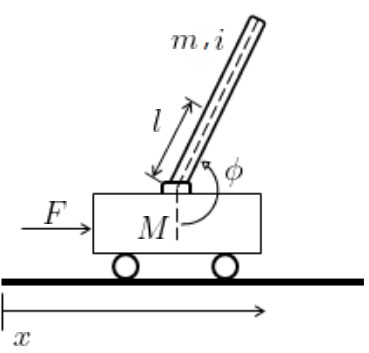
After modeling, using the free body diagram and the summation of forces, two equations are determined to describe the behavior of the system. In order to control the system, the two equations must be linearized. The linearization will be about the desired point of equilibrium. This point is \theta = \phi. Considering \phi a small deviation of the equilibrium point, the position of the pendulum may be represented by \theta = \pi + \phi The following approximations are used:
cos\theta \approx -1
sin\theta \approx -\phi
\dot{\theta^{2}} = \dot{\phi^{2}} = 0
Using the linearization, the following equations can be written:
\(I+ml^{2} \) \ddot{\phi} - mgl \phi = ml\ddot{x}
\(M+m \) \ddot{x} + b\dot{x} - ml \dot{\phi} = F
In order to write the transfer function it is necessary to apply the Laplace Transform to the equiations. The new equations are:
\(I+ml^{2} \) \phi (s)s^{2} - mgl \phi (s) = mlX(s)s^{2}
\(M+m \)X(s)s^{2} + bX(s)s^{2} - ml \phi (s)s^{2} = F(s)
Combining the two equations, the two transfer functions – position of the pendulum and position of the cart with respect to the force – are determined.
|




 Where:

