fechar
fechar

The Root Locus Method

The settling time t_{s} (0.2% criterion):

t_{s} = 0.5s ~ \rightarrow ~ t_{s} = \frac{4}{\sigma} ~ \rightarrow ~ \sigma = \frac{4}{0.5} ~ \rightarrow ~ \sigma = 8

This information can be obtained from the Root Locus Plot:


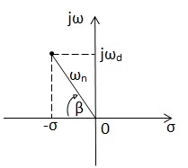
s = - \sigma \pm j \omega_{d}
\omega_{d} = \omega_{n} \sqrt{1-\zeta^2}
\sigma = \zeta ~ \omega_{n}
cos \beta = \zeta


From the Root Locus Plot, a point of σ = -0,8 is found. If there is a point whose real part is -8 (zoom the plot near the region of interest to find a more accurate location for the point) and keeping in mind that all the points of a Root Locus Plot obey the relation:

1 + K. G(s)C(s) = 0

The gain, K, can be computed. Other information can be computed as well.


SIMULAÇÕES EM ENGENHARIA ELÊTRICA


detalhes


INVERTED PENDULUM

ADJUSTMENT OF THE CONTROLLER USING THE ROOT LOCUS METHOD

Another method to analyze the stability is the Root Locus Méthod .It allows the trajectories of the locations of the roots of a polynomial on the complex plane when a parameter varies. In the case under consideration, the parameter is the gain K.

Given the parameters of the system and tha gains of the PID controller, the Root Locus Plot can be drawn.

M= kg     I=     kg.m²m= kg     g= 9.8 kg.m/s^2

b= N/m/s    l=m     K_{P}=    K_{I}=   K_{D}=


Real axis from to   Imaginary axis from to

The use of the Root Locus Method allows the adjustment of the controller to comply with some specifications. One example is the settling time to be 0.5s (0.2% criterion).

For additional information on the Root Locus Method, click on the magnifying glass.

The gain, K, associated to any point of the Root Locus Plot can be computed:

Point = + j

The impulse response of the system (when the gain is K) can be computed:

K =


voltar